Please note that this page is outdated!
If you are interested in the spike detection code, please refer to my new page and follow the "Software" link, or go directly to
the updated page.
 Previous.
The problem of detecting transient signals given a collection of noisy
observations has been studied for decades. The presence of a useful signal
in a background noise is normally cast as a hypothesis testing, where under
the null hypothesis no signal is present.
If the signal to be detected is
not perfectly known, usually no uniformly most powerful (UMP) test
exists, and the performance of a detector depends on
signal representation. In general, a signal representation can be model
based and expansion based. When no apropriate model for the signal can be
found,
one usually resorts to a "canonical set" of basis function where the signal
is
projected, giving rise to expansion coefficients. We can think of these
coefficients as of signal representation in a new coordinate system.
Depending on the signal representation the
detection problem can be formulated in different domains such as time domain,
frequency domain and time-frequency domain. In time-frequency domain, a
signal is projected onto a basis of waveforms that are well localized
(subject to Hiesenberg uncertainty principle) in both
time and frequency, yielding a two-dimensional signal
representation Tx(w,t) of a one-dimensional signal
x(t).
An example of this
representation is a windowed Fourier
transform introduced by
Gabor. A
breakthrough in the theory of wavelets offered
a powerful alternative to windowed Fourier transform, where a one-dimensional
signal
x(t) is represented in time-scale domain by virtue of a wavelet
transform Tx(a,b).
Previous.
The problem of detecting transient signals given a collection of noisy
observations has been studied for decades. The presence of a useful signal
in a background noise is normally cast as a hypothesis testing, where under
the null hypothesis no signal is present.
If the signal to be detected is
not perfectly known, usually no uniformly most powerful (UMP) test
exists, and the performance of a detector depends on
signal representation. In general, a signal representation can be model
based and expansion based. When no apropriate model for the signal can be
found,
one usually resorts to a "canonical set" of basis function where the signal
is
projected, giving rise to expansion coefficients. We can think of these
coefficients as of signal representation in a new coordinate system.
Depending on the signal representation the
detection problem can be formulated in different domains such as time domain,
frequency domain and time-frequency domain. In time-frequency domain, a
signal is projected onto a basis of waveforms that are well localized
(subject to Hiesenberg uncertainty principle) in both
time and frequency, yielding a two-dimensional signal
representation Tx(w,t) of a one-dimensional signal
x(t).
An example of this
representation is a windowed Fourier
transform introduced by
Gabor. A
breakthrough in the theory of wavelets offered
a powerful alternative to windowed Fourier transform, where a one-dimensional
signal
x(t) is represented in time-scale domain by virtue of a wavelet
transform Tx(a,b).
Software
All files are MATLAB® M-files or MAT-files. You will need Wavelet Toolbox
installed in order to execute the main function.
detect_spikes_wavelet.m (6.6 KB)
get_score.m (1.4 KB)
lag_ts.m (0.7 KB)
lead_ts.m (0.7 KB)
clean.mat (160 KB)
corrupted.mat (160 KB)
Tutorial
detect_spikes_wavelet is a stand-alone function for detection of
neural transients in noisy data. The other files are for tutorial purposes
only.
>> load clean.mat

>> who


Your variables are:


Signal
Your workspace now contains a variable Signal,
which is a row vector of neural
data to be analyzed. This data is artififially created, and contains 10 equally
spaced spikes (transients). The attribute "clean" indicates that the data
does not contain any noise. You can visualize the signal by
>> plot(Signal)

>> set(gca,'XLim',[1 length(Signal)],'YLim',[-3 3])
The produced figure is shown below (click on the figure for full size image)
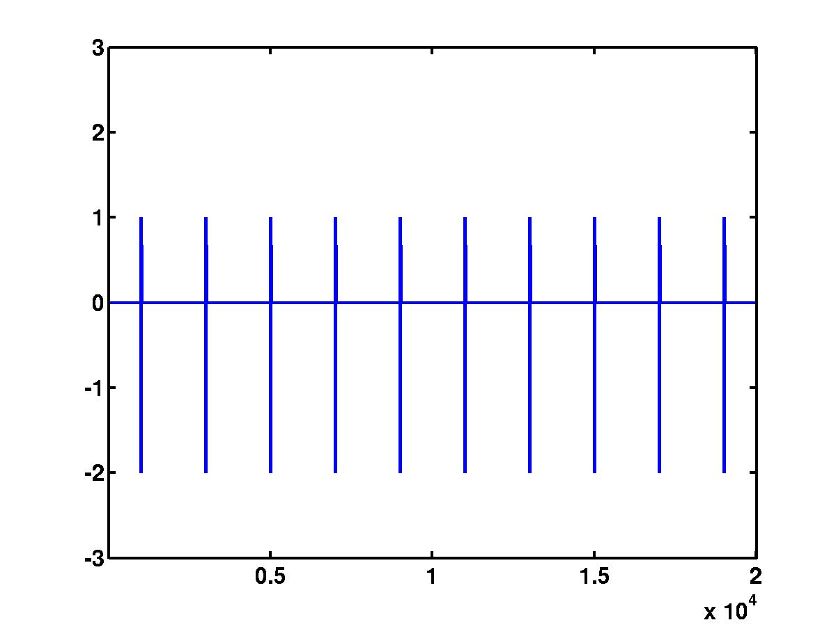
The sampling rate of the generated signal is 20 [kHz], so the figure
corresponds to 1 second of data.
Close inspection of individual spikes shows that they consist of two sinusoid
semicycles of different amplitudes. The "width" of the spikes is set to 0.6
[msec]. Running the detection algorithm on Signal
is not particularly
challenging, but reveals the true times of spike occurrences.
>> TT=detect_spikes_wavelet(Signal,20,[0.5 1.0],'reset',0.1,'bior1.5',1,1)

wavelet family: bior1.5

10 spikes found

elapsed time: 1.7704

TT =

   Columns 1 through 6

     1003   3003   5003   7003   9003        11003

    Columns 7 through 10

     13003   15003   17003    19003
The last two arguments in the function are plot and comment flags. To supress
comments and plots, you should pass a number different from 1, for example
>> TT=detect_spikes_wavelet(Signal,20,[0.5 1.0],'reset',0.1,'bior1.5',0,1);
produces comments but not plots, and
>> TT=detect_spikes_wavelet(Signal,20,[0.5 1.0],'reset',0.1,'bior1.5',1,0);
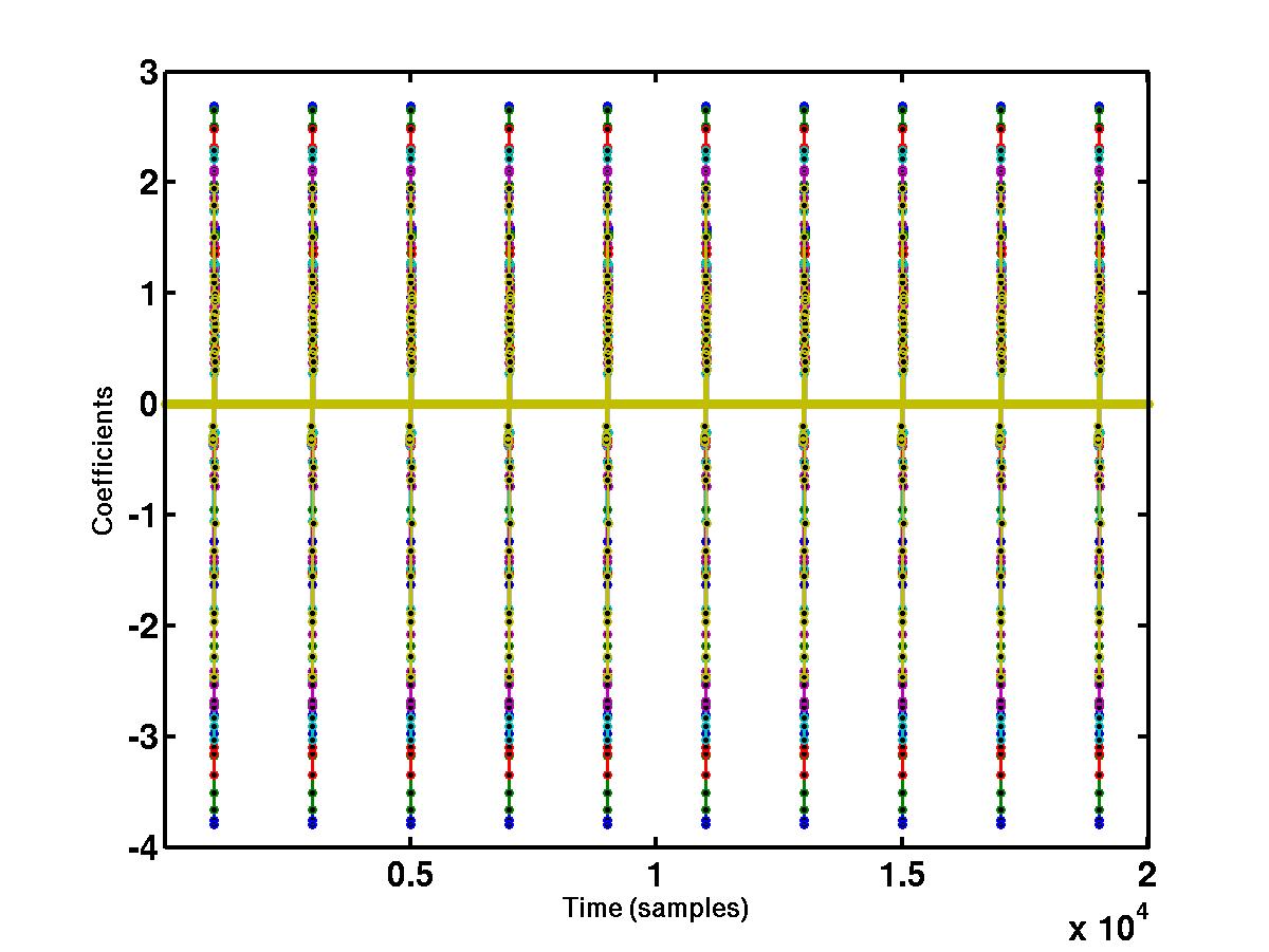
produces plots but not comments. If you opt for plots, the program generates
two figures which are shown below.
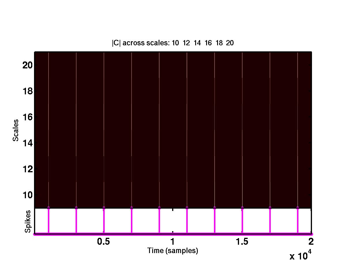
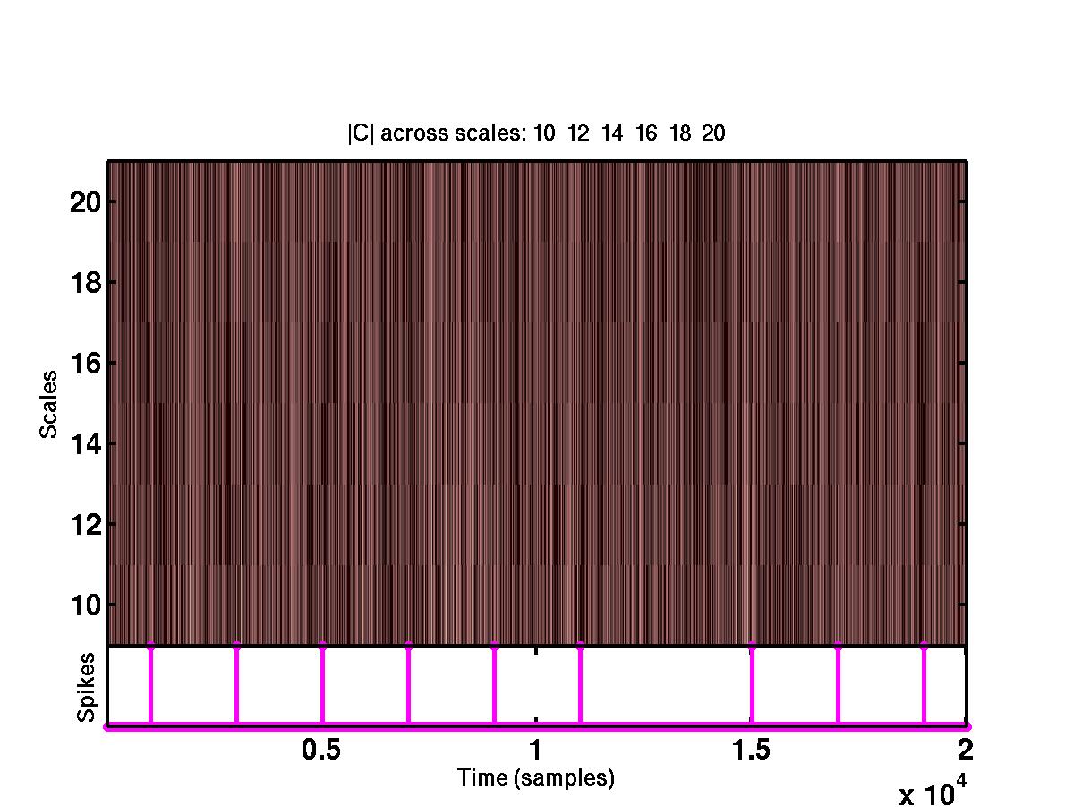
The upper plot shows the time-scale representation of the signal, where the
absolute values of wavelet coefficients are color coded. At the bottom of
the same plot are the locations of the detected spikes. By looking at the full
size version of this figure, it is obvious that the spikes correspond to
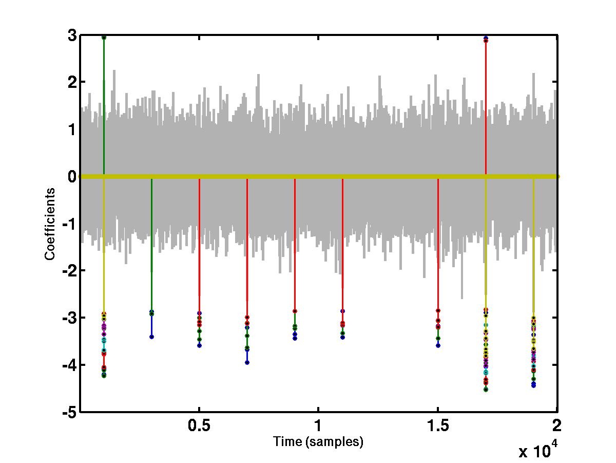
"large" coefficients across different scales. The bottom figure shows the
wavelet coefficients at
different scales that cross a detection threshold. The coefficients at
different scales are represented by different colors, e.g red, blue, green
etc. The coefficients that do not cross the detection threshold are shrunk to
0.
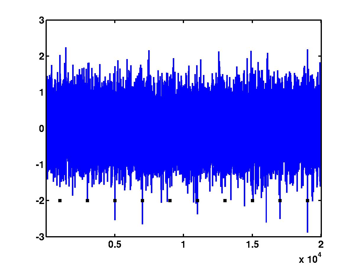
We now take the time series from above and corrupt it by an additive white
noise, with a standard deviation determined from desired signal-to-noise
ratio (SNR).
>> load corrupted.mat

>> plot(Signal)

>> set(gca,'XLim',[1 length(Signal)],'YLim',[-3 3])
In the outcome of the code above, we obtain the figure of the noisy spike
train (see below). Black squares indicate the positions of the spikes.
Clearly, a
simple detection based on amplitude thresholding could not detect "short"
spikes (spikes 1, 5 and 7) without accepting a number of false positives.
Then, we detect the spikes in the noisy data by
>> TE=detect_spikes_wavelet(Signal,20,[0.5 1.0],'reset',0.1,'bior1.5',1,0);
which results in the following figures:
As can be seen from the figure above, one of the spikes (spike 7) was not detected. This can be verfied by running the function get_score.m which
returns the number of correctly detected spikes, the number of omissions as well as the number of false positives. Indeed,
>> get_score(TT,TE,20)

ans =

         9       1       0
indicating that there are 9 correctly detected spikes, 1 omission and 0 false positives. You can trade-off omissions and false positives by varying the parameter L (type help detect_spikes_wavelet to learn more about this
parameter), i.e.
>> TE=detect_spikes_wavelet(Signal,20,[0.5 1.0],'reset',0.0,'bior1.5',0,0);

>> get_score(TT,TE,20)

ans =

          9        1        3

>> TE=detect_spikes_wavelet(Signal,20,[0.5 1.0],'reset',-0.03,'bior1.5',0,0);


>> get_score(TT,TE,20)

ans =

         10        0         4
You can now play with different choice of wavelet functions, such as
'bior1.3' 'db2' 'haar' etc., and compare their performances.