


Next: Simulation Results
Up: Decoding From Spike Trains
Previous: Detection Problem
The goal of this section is to present a decoding method that utilizes full
statistical description of the response  . In this context the equation
(1) becomes
. In this context the equation
(1) becomes
![\begin{equation*}{\begin{split}&P(x_i(t) \vert S(t))=\frac{P(S(t) \vert x_i(...
... s_2(t), \cdots,s_N(t)] \vert x_i(t)) P(x_i(t))} \end{split}}\end{equation*}](img21.png) |
(3) |
The proposed scheme is fairly general and often difficult to implement. To make
the problem tractable and easy to implement we will make several important
assumptions.
Assumption The responses of individual neurons are statistically
independent. The consequence of this assumption is that
![$\displaystyle P([s_1(t), s_2(t), \cdots,s_N(t)] \vert x_i(t))=\prod_{j=1}^{N} P(s_j(t) \vert x_i(t))$](img22.png) |
(4) |
Assumption The prior probabilities of individual inputs are equal i.e.
 |
(5) |
Applying (4) and (5) to the decoding scheme
(3) we have
![$\displaystyle P(x_i(t) \vert [s_1(t), s_2(t), \cdots,s_N(t)])= \frac{{\dis...
...,x_i(t))} {\displaystyle{\sum_{i=1}^M}\prod_{j=1}^{N} P(s_j(t) \vert x_i(t))}$](img24.png) |
(6) |
The chief difficulty of decoding in the present context is determining the
conditional probability of
 th response given
 th input.
Let
 be the response of the
th neuron in the population to the input
be the response of the
th neuron in the population to the input  . Our goal is to
evaluate the conditional probability
. Our goal is to
evaluate the conditional probability
 . Since we
consider only one input-response pair at a time, the indices
. Since we
consider only one input-response pair at a time, the indices  and
and  will
be dropped for simplicity. The signal
will
be dropped for simplicity. The signal
 is fully characterized by the sequence of times
 so we have
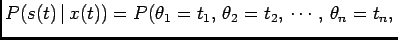 no spikes in no spikes in![$\displaystyle [t_n, t] \vert x(t)),$](img34.png) |
|
where  is a random variable that corresponds to the arrival time of
the
is a random variable that corresponds to the arrival time of
the
 th spike in the spike train. Clearly, is a continuous
random variable, so the probability of the event above is equal to 0, and
we are better off with its likelihood (probability density function), defined
by
th spike in the spike train. Clearly, is a continuous
random variable, so the probability of the event above is equal to 0, and
we are better off with its likelihood (probability density function), defined
by
where conditioning on  has been dropped for simplicity and
![$ N_{[t_n+dt_n, t]}=0$](img38.png) means that we have no spikes on the interval
means that we have no spikes on the interval
![$ [t_n+dt_n, t]$](img39.png) .
.
Assumption The arrivals (non-arrivals) at instant  are only dependent
on the previous arrival. This Markov-type assumption means that
are only dependent
on the previous arrival. This Markov-type assumption means that  depends on
 only.
only.
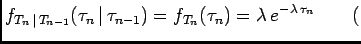
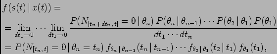
Under this assumption the conditional probability calculation further
simplifies to
and the probability density function (pdf) becomes
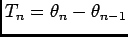
where
 represent transition densities.
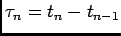
It is often more useful to use interspike intervals (ISI) defined by
represent transition densities.
It is often more useful to use interspike intervals (ISI) defined by
 (
(
 ) instead of spike arrivals
. The conditional density then becomes
) instead of spike arrivals
. The conditional density then becomes
where
 (
( ) and
) and  is a normalization constant that makes
 a valid pdf candidate. The transition densities
 are to be found using either parametric or non-parametric
methods. Parametric methods rely on assuming the transition densities are
parameterized by a number of unknown parameters which are found from
experimental observations. Non-parametric methods rely on direct (pointwise)
estimate of the transition densities. Both methods are based on experimental
data. Using densities instead of probabilities
the decoding algorithm (6) becomes
are to be found using either parametric or non-parametric
methods. Parametric methods rely on assuming the transition densities are
parameterized by a number of unknown parameters which are found from
experimental observations. Non-parametric methods rely on direct (pointwise)
estimate of the transition densities. Both methods are based on experimental
data. Using densities instead of probabilities
the decoding algorithm (6) becomes
![$\displaystyle f(x_i(t) \vert [s_1(t), s_2(t), \cdots, s_N(t)])= \frac{{\di...
..._i(t))} {{\displaystyle \sum_{i=1}^{M}\prod_{j=1}^{N}}f(s_j(t) \vert x_i(t))}$](img54.png) |
(7) |
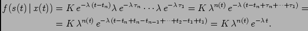
To illustrate the application of the algorithm above, let us suppose that
the underlying spike generating mechanism is a Poisson process with a
constant rate  . One can easily show that
 renewal assumption renewal assumption |
|
In particular one has
To signify that the rate depends on both input and cell, we write
where
 and
and
 is so-called tuning curveof the
th cell. One can easily show that in this case
is so-called tuning curveof the
th cell. One can easily show that in this case
 .
Written more detailed, the conditional pdf is given
by
.
Written more detailed, the conditional pdf is given
by
and finally the decoding scheme (7) simply becomes
![$\displaystyle f(x_i(t) \vert [s_1(t), s_2(t), \cdots, s_N(t)])= \frac{{\di...
...rod_{j=1}^{N}} \frac{[\Lambda_j(x_i)]^{n_j(t)}}{n_j(t)!}e^{-\Lambda_j(x_i) t}}$](img64.png) |
(8) |
This result coincides with decoding scheme based on firing rates only. Namely,
if  is the number of spikes fired by the
th cell on the
interval
is the number of spikes fired by the
th cell on the
interval ![$ [0, t]$](img9.png) , one can rewrite (7) as
, one can rewrite (7) as
![$\displaystyle P(x_i(t) \vert [n_1(t), n_2(t), \cdots, n_N(t)])= \frac{\prod P(n_j(t) \vert x_i(t))} {\sum\prod P(n_j(t) \vert x_i(t))},$](img65.png) |
(9) |
and
Finally (9) becomes
![\begin{displaymath}\begin{split}&P(x_i(t) \vert [n_1(t), n_2(t), \cdots, n_...
...a_j(x_i)]^{n_j(t)}}{n_j(t)!}e^{-\Lambda_j(x_i) t}} \end{split}\end{displaymath}](img67.png) |
(10) |
which is result identical to (8). This result is not surprising since
Poisson process is completely determined by the rate and taking into
account full statistical description of the spike trains does not yield
any new information.
Next: Simulation Results
Up: Decoding From Spike Trains
Previous: Detection Problem
Zoran Nenadic
2002-07-18
![\begin{displaymath}\begin{split}&f(s(t) \vert x(t))\triangleq\frac{\partial^n ...
...n+dt_n], N_{[t_n+dt_n, t]}=0)}{dt_1\cdots dt_n}, \end{split}\end{displaymath}](img37.png)
![\begin{displaymath}\begin{split}P(s(t) \vert x(t))&=P(N_{[t_n+dt_n, t]}=0 \v...
...})\cdots P(\theta_2 \vert \theta_1) P(\theta_1), \end{split}\end{displaymath}](img43.png)
![\begin{displaymath}\begin{split}&f(s(t) \vert x(t))=\ &=K P(N_{[t_n, t]}=0...
...vert T_1}(\tau_2 \vert \tau_1) f_{T_1}(\tau_1), \end{split}\end{displaymath}](img48.png)
![$\displaystyle f(s_j(t) \vert x_i(t))=\frac{[\Lambda_j(x_i)]^{n_j(t)}}{n_j(t)!} e^{-\Lambda_j(x_i) t},$](img63.png)
![$\displaystyle P(n_j(t) \vert x_i(t))=\frac{[\Lambda_j(x_i) t]^{n_j(t)}}{n_j(t)!} e^{-\Lambda_j(x_i) t}.$](img66.png)