In the spirit of detection problem defined by equation
(2), let us assume
that ![]() takes its values from the set
takes its values from the set
![]() (
(![]() ). For each
). For each
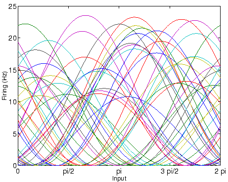
![]() and for each neuron from the population, the mean firing rate
and for each neuron from the population, the mean firing rate
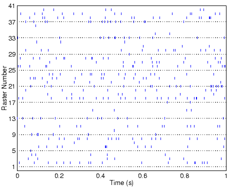
![]() is calculated according to (11), and sequences of spikes
are generated using Poisson generator with dead time
is calculated according to (11), and sequences of spikes
are generated using Poisson generator with dead time
![]() ms. The
realization of one such collection of random processes is given by
Fig. 3. The raster plots from Fig. 3 correspond to one
of the eight inputs from
ms. The
realization of one such collection of random processes is given by
Fig. 3. The raster plots from Fig. 3 correspond to one
of the eight inputs from
![]() . Given a conditional response, such as
the one shown by Fig. 3, our goal is to estimate the most likely
value of the input that elicited such response. Since we know what inputs are
indeed behind every response, we can use this knowledge for cross-validation of
our results. The decoding is performed according to (7).
. Given a conditional response, such as
the one shown by Fig. 3, our goal is to estimate the most likely
value of the input that elicited such response. Since we know what inputs are
indeed behind every response, we can use this knowledge for cross-validation of
our results. The decoding is performed according to (7).
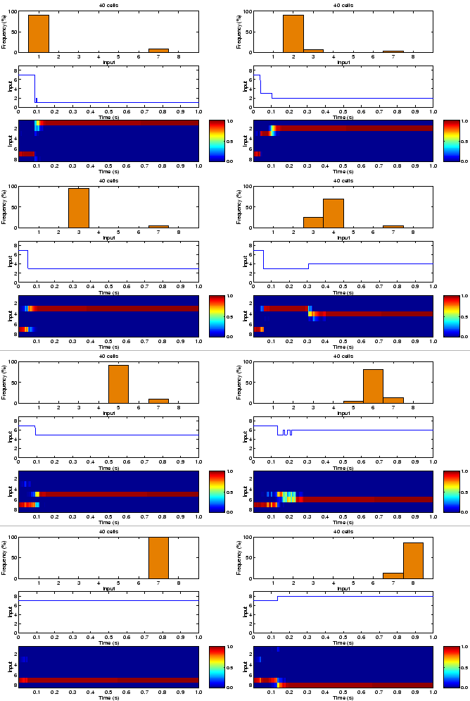
The results of the decoding procedure across 8 inputs are shown in
Fig. 4. The top plot in each subfigure shows the relative frequency
of decoded directions. It is not surprising that the decoded input changes
in time, despite the fact that the encoded input is constant in time. However,
the decoded value stabilizes after some time, and does not change any more. The
settling time is different for different inputs, e.g. 300 ms for input 4
(
![]() ). The middle plot in each subfigure shows the traces of
decoded inputs as a function of time.
Input 7 is decoded with a 100
). The middle plot in each subfigure shows the traces of
decoded inputs as a function of time.
Input 7 is decoded with a 100![]() accuracy, i.e. this input emmerges as
dominant (most likely) for all times. The bottom image in each subfigure shows
the color coded likelihood of each input. The colorbar indicates that the
likelihoods are normalized between 0 and 1.
accuracy, i.e. this input emmerges as
dominant (most likely) for all times. The bottom image in each subfigure shows
the color coded likelihood of each input. The colorbar indicates that the
likelihoods are normalized between 0 and 1.